The Low Volatility Factor: A Steady Approach
Introduction
Here’s a simple idea: stocks that move less tend to deliver better risk-adjusted returns than those with wild price swings. It’s a pattern that shows up in equities and other asset classes too.
This is the first in a series on cross-sectional stock selection. I’m starting with a single-factor strategy, then I’ll gradually build up: combining multiple signals with linear regression, testing different design choices, and later exploring non-linear models like LightGBM. At the end, I’ll compare everything to see if complexity actually helps. But first, let’s keep it simple and see how far a basic low-volatility sort can take us.
Tradeable Universe
I’m using the Russell 1000 (RIY), which tracks the largest U.S. stocks. To keep things realistic, I filter out stocks priced under $5. The data runs from 1995 to 2024, covering around 3,300 stocks as companies enter and exit the index. At any given time, about 1,000 stocks are tradeable. Since I’m using point-in-time constituents, there’s no survivorship bias. Figure 1 shows how many tradeable stocks there are over time.

Figure 1: Number of tradeable stocks over time.
Measuring Volatility
To find low-volatility stocks, I compute the standard deviation of daily returns—basically measuring how much a stock’s price bounces around. I use three short-term rolling windows:
- 5 trading days
- 10 trading days
- 21 trading days
Shorter windows react more quickly to changes in market conditions, while longer windows provide more stable estimates. By combining them, I aim for a volatility signal that’s both responsive and robust.
Volatility is computed as:
\[\hat{\sigma}_{i,t} = \sqrt{\frac{1}{N,1} \sum_{j=1}^N \left( r_{i,t,j} , \bar{r}_{i,t} \right)^2}\]where $r_{i,t}$ is the daily return of stock $i$ at time $t$, and $N$ is the length of the rolling window. I annualize this by multiplying the daily volatility by $\sqrt{252}$, assuming 252 trading days in a year.
Across the dataset, the average annualized volatility is about 33%, with most stocks falling between 18% and 39%. The median is 26%. A few names have extreme swings, so I winsorize the volatility values at 5% and 200% to prevent outliers from distorting the rankings.
As shown in Figure 2, the distribution is right,skewed: most stocks cluster around moderate volatility levels, but a small number show very high fluctuations.

Figure 2: Distribution of annualized volatility across all stocks.
Does Low Volatility Matter?
I wanted to see if low-volatility stocks actually behave differently, so I looked at their returns over the next 10 trading days. I checked two things: raw returns and risk-adjusted returns (using the Sharpe ratio).
The correlation between volatility and raw return came out slightly positive, around 0.03. So more volatile stocks seemed to perform a bit better—at least at first glance. That wasn’t what I expected, but it’s a small effect. When I switched to Spearman correlation (which handles outliers better), it flattened out to zero.
Things change when I look at Sharpe ratios. Here, the correlation with volatility was negative: -0.035 with Pearson, and -0.04 with Spearman. So while high-vol stocks might deliver bigger returns sometimes, they do it with way more noise. On a risk-adjusted basis, they come out worse.
The signal is weak, but that’s normal for this stuff. What matters is that it shows up consistently, especially when you apply it across a large universe.
Sorting Stocks into Portfolios
To turn this into a tradeable strategy, I rank stocks by volatility at each point in time and sort them into five portfolios. This ensures that portfolio assignments are always relative to the current market.
Here’s how it works:
- Compute rolling volatility for each stock.
- Rank stocks by volatility within the universe.
- Normalize ranks to a 0,1 scale.
- Assign stocks to one of five portfolios based on percentile rank.
Let $r_{i,t}$ be the cross-sectional rank of stock $i$ at time $t$, and $N$ be the number of stocks. The normalized rank is:
\[\frac{r_{i,t}}{N}\]Stocks are then grouped into these buckets:
- Portfolio 1: Lowest 10% of stocks ($0 \leq \text{Rank Score} < 0.1$) → Low volatility
- Portfolio 2: 10% to 20% of stocks ($0.1 \leq \text{Rank Score} < 0.2$)
- Portfolio 3: 20% to 80% ($0.2 \leq \text{Rank Score} < 0.8$)
- Portfolio 4: 80% to 90% of stocks ($0.8 \leq \text{Rank Score} < 0.9$)
- Portfolio 5: Highest 10% ($0.9 \leq \text{Rank Score} \leq 1.0$) → High volatility
This way, every stock’s classification is determined relative to the cross-sectional volatility of the market at that time.
Portfolio Construction
Once the stocks are grouped into buckets, I construct two types of portfolios: one that assigns equal weights to each stock, and another that adjusts weights to target a specific volatility level.
1. Equal,Weighted Portfolio
In the equal-weighted portfolio, each stock receives the same weight:
\[w_{i,t} = \frac{1}{N_t}\]where \(N_t\) is the number of stocks in the portfolio at time \(t\). The portfolio remains fully invested. To create the long-short strategy, I go long the low-volatility portfolio (P1) and short the high-volatility portfolio (P5), using equal weights on both sides.
This setup introduces a problem: the two legs have different levels of volatility. Low,volatility stocks naturally exhibit less risk, so the short leg tends to dominate in terms of exposure. This imbalance reduces the effectiveness of the strategy on a risk-adjusted basis.
2. Volatility,Targeted Portfolio
To correct for this imbalance, I use volatility targeting. The idea is to scale the weight of each stock based on its volatility relative to a fixed target. The scaling factor is defined as:
\[\alpha_{i,t} = \frac{\sigma_{\text{target}}}{\hat{\sigma}_{i,t}}\]where:
- \(\sigma_{\text{target}} = 20\%\) is a fixed target volatility level
- \(\hat{\sigma}_{i,t}\) is the estimated future volatility of stock \(i\), computed using a 60-day rolling standard deviation
Each stock’s weight becomes:
\[w_{i,t} = \frac{1}{N_t} \cdot \alpha_{i,t}\]This approach increases the weight of stocks with below,target volatility and reduces the weight of those above it. To avoid excessive concentration, I cap individual weights at 4%. The total portfolio weight is also constrained to remain below or equal to 1.0.
During periods of high volatility, the portfolio may become partially invested to stay within the exposure limit. This isn’t market timing,it’s a way to control portfolio,level risk dynamically.
Portfolios are rebalanced weekly based on updated volatility estimates. Transaction costs are not included in this analysis.
Results
Equal,Weighted Portfolio
I start by evaluating the equal-weighted version of the strategy. The long side holds the lowest,volatility stocks (P1), and the short side holds the highest,volatility ones (P5). Within each group, stocks are given equal weight.
On their own, the results make sense. The low-volatility portfolio delivers a geometric return of 11.8% with a Sharpe ratio of 1.0. The high-volatility portfolio returns 4.7%, with much higher volatility and little risk-adjusted performance.
But when combining the two into a long-short portfolio, the performance breaks down. The issue is a volatility mismatch: the short side is much more volatile than the long side,38.6% versus 12.2%. Equal weighting doesn’t account for this difference. As a result, the short leg ends up driving most of the portfolio’s risk.
The final long-short portfolio has high volatility (32.6%), a negative Sharpe ratio (-0.2), and a drawdown over 90%. Figure 3 shows the key performance metrics before applying volatility targeting. A full summary is included in Table 1.
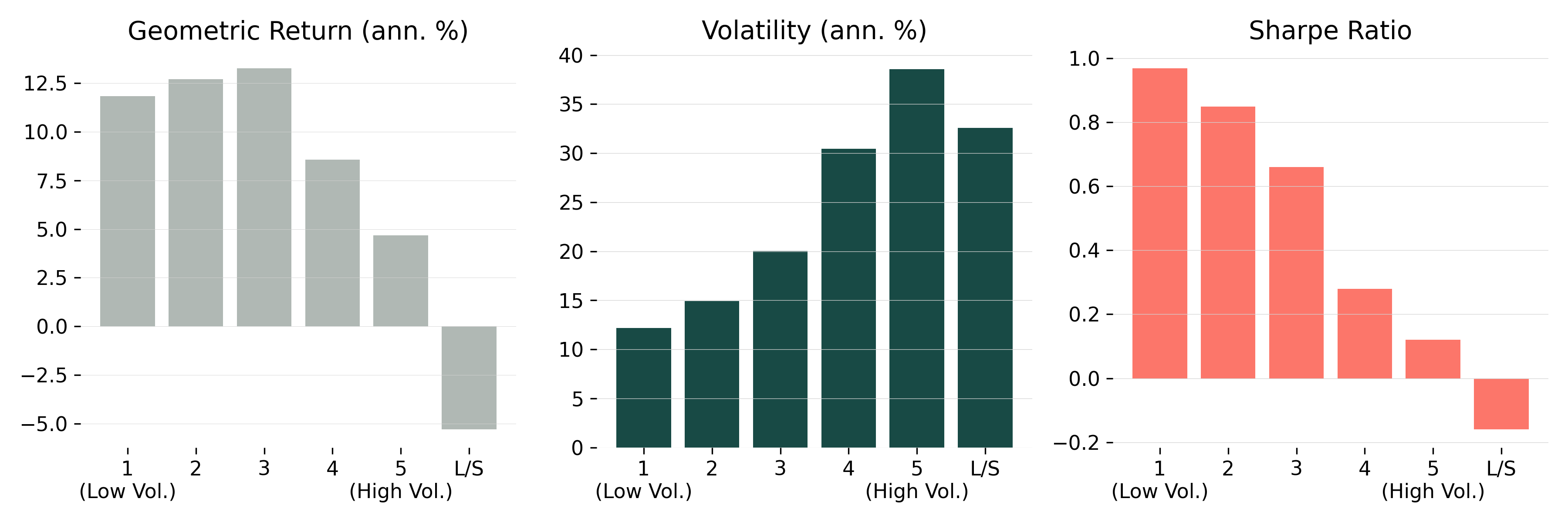
Figure 3: Geometric Return, Volatility, and Sharpe Ratio for equal-weighted portfolios (before volatility targeting).
Volatility,Targeted Portfolio
Volatility targeting adjusts for the imbalance between long and short legs by scaling each stock’s weight relative to a fixed volatility target (set here at 20%). This helps align the total risk of the long and short portfolios and results in more stable performance.
After applying volatility targeting, the improvements are clear. The long-short portfolio volatility drops from 32.6% to 8.3%, and the Sharpe ratio rises from -0.2 to 0.9. The max drawdown is also cut significantly,from over 90% to 33.6%.
The long,only portfolio becomes slightly more stable as well. Its volatility decreases from 12.2% to 9.7%, while the Sharpe ratio improves from 1.0 to 1.1.
Figure 4 shows how volatility, return, and Sharpe ratio change across the five portfolios after targeting is applied. The result is more balanced exposure and better overall risk-adjusted returns.
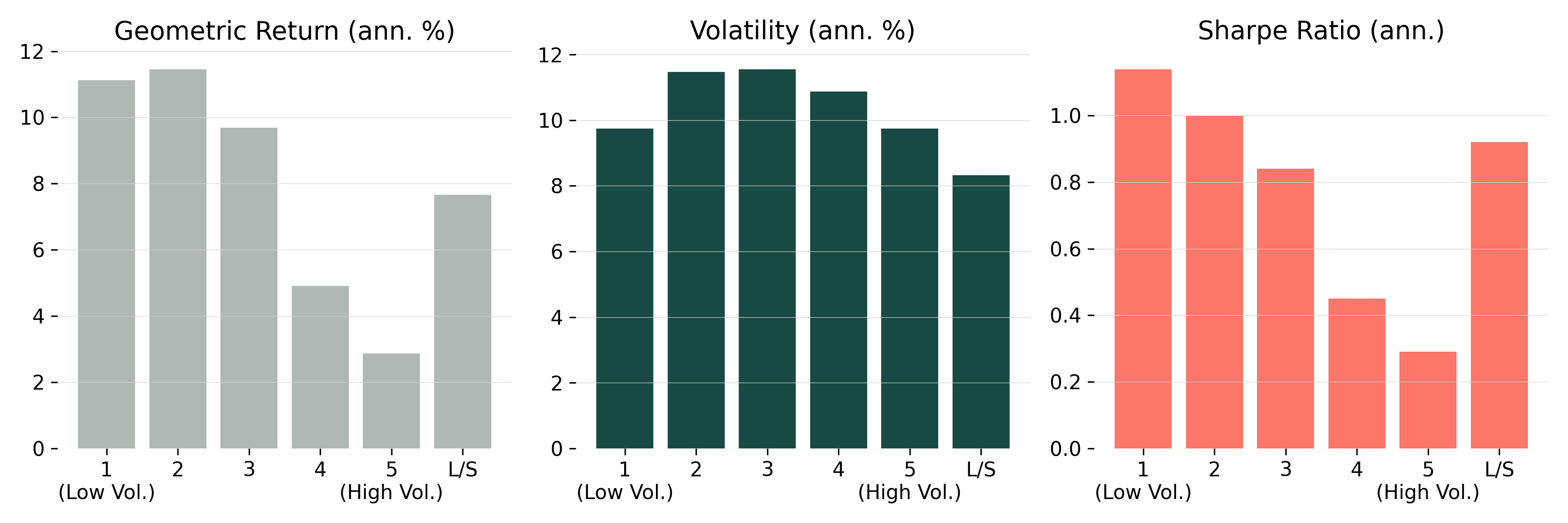
Figure 4: Geometric return, volatility, and Sharpe ratio after volatility targeting.
Performance Over Time
The impact of volatility targeting is also visible over time. Figure 5 shows the net asset value of the long-short portfolio after adjustment. Compared to the equal-weighted version, returns are smoother and drawdowns less severe.
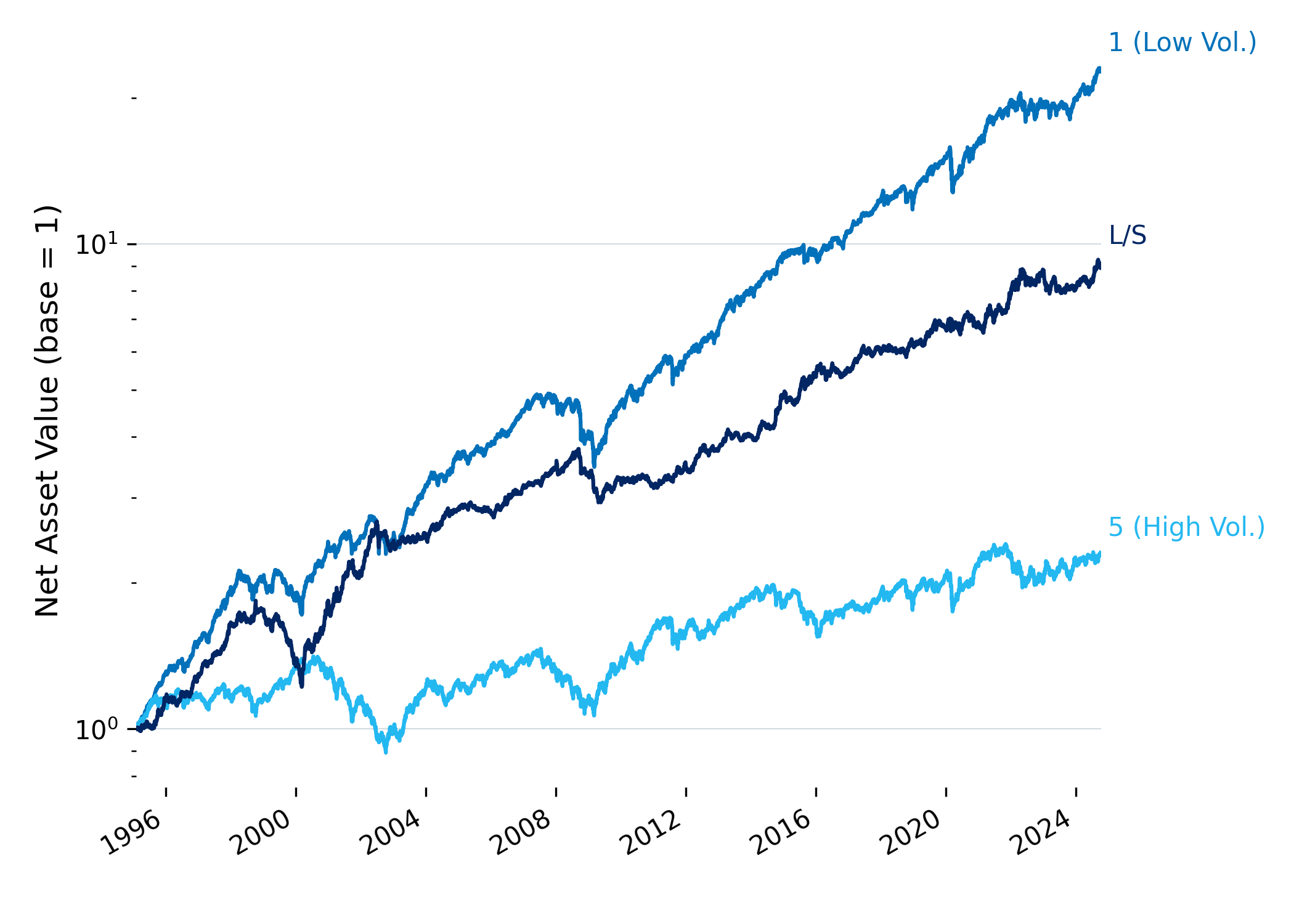
Figure 5: Net asset value of the volatility,targeted long-short portfolio.
Summary Table
To summarize the improvements, here are the core metrics before and after applying volatility targeting:
| Metric | Long (No VT) | Long (VT) | Short (No VT) | Short (VT) | L/S (No VT) | L/S (VT) |
|---|---|---|---|---|---|---|
| Geometric Return | 11.8% | 11.1% | 4.7% | 2.9% | -5.3% | 7.7% |
| Volatility | 12.2% | 9.7% | 38.6% | 9.7% | 32.6% | 8.3% |
| Sharpe Ratio | 1.00 | 1.14 | 0.12 | 0.30 | -0.19 | 0.93 |
| Max Drawdown | 40.2% | 29.5% | 89.6% | 36.7% | 91.6% | 33.6% |
| Max Time Underwater | 863 days | 612 days | 4,802 days | 1,647 days | 5,539 days | 944 days |
Table 1: Performance metrics before and after volatility targeting. “VT” applies volatility targeting; “No VT” uses equal weighting.
Portfolio Exposure Over Time
Figure 6 shows how total portfolio weights evolve over time for both the long (low-volatility) and short (high-volatility) sides after applying volatility targeting.
By total weight, I mean the sum of all individual stock weights within each leg. Since the short side holds more volatile stocks, it naturally receives less capital,typically between 0.2 and 0.6. The long side, made up of more stable names, stays closer to fully invested.
This behaviour is expected. Volatility targeting reduces exposure to riskier assets and increases it for more stable ones. During periods of market stress,like the dot,com crash, the financial crisis, or COVID,both legs reduce their exposure. The mechanism reacts by shrinking position sizes to stay within the target risk level.
The result is a portfolio that adapts to changing market conditions without needing explicit market timing.

Figure 6: Total weight of all positions in the long (P1) and short (P5) portfolios after volatility targeting.
Conclusion
The low-volatility factor delivers stronger risk-adjusted returns. Lower,vol stocks tend to outperform, which goes against the usual link between higher risk and higher return.
Equal weighting in a long-short setup creates a risk imbalance. The short leg ends up dominating volatility, which pulls down performance. Volatility targeting fixes that imbalance by adjusting weights to align the risk on both sides, making the strategy more stable and improving Sharpe ratios.
Even this simple adjustment already helps a lot. In the next post, I’ll look at how combining multiple signals can take things a step further.