Multi-Factor Stock Selection with Ridge Regression
Introduction
In the last article I showed how scaling returns by volatility helped improve performance with minimal complexity. This time I want to let the model learn how to combine different features instead of me setting the rules manually.
Stock prediction is hard. Instead of trying to guess exact returns, I’m focusing on something more practical: figuring out whether stock A will perform better than stock B. I don’t need to know by how much—just which one is likely to do better.
I’m using a multiple linear regression model that takes in many features (like price changes, trading volume, and risk levels) and learns how to weigh them. The model is trained on a target label—basically the outcome I want it to predict, like future returns or the Sharpe ratio.
But there are a few challenges. Features behave differently over time: their distributions shift, patterns that worked before can break down, and some signals that seem useful in one market environment might completely disappear in another. On top of that, the signal-to-noise ratio is low, making it tough to extract meaningful insights.
Data
I’m using the same dataset as the previous article: daily price, volume, and market cap data for all Russell 1000 (RIY) constituents, covering about 3,300 stocks historically. I use point-in-time constituents and filter out stocks priced below $5 to keep things realistic.
Feature Engineering
I come from a stats and CS background, so I naturally lean toward letting the data figure out relationships rather than imposing assumptions. This is different from traditional multifactor approaches where you manually decide how to combine features. Instead, I use a regression model that learns the feature weights directly from the data.
For now, I’m keeping it simple with linear regression—assuming relationships are linear and avoiding interaction terms. It’s a straightforward approach that focuses on finding direct connections between features and the target.
Choosing Predictive Features
Before the model can learn anything useful, I need to define the right features and pick a target variable. I focus on price, volume, market cap, and market-derived indicators, computing them daily for all 3,300 stocks in my universe. Here’s what I’m using:
1. Momentum Features
These capture trend-following behavior.
- Lagged returns over 1 to 10 days
- Rolling cumulative returns over 21 to 252 days
- MACD to detect momentum shifts
2. Volatility Features
These measure risk.
- Rolling historical volatility over 21, 63, or 126 days
- Average True Range (ATR) to normalize price fluctuations
3. Liquidity Features
These assess trading activity.
- Rolling mean and standard deviation of trading volume
- Ratio of current volume to its rolling maximum to spot unusual activity
4. Size Features
These measure company scale.
- Rolling mean and minimum of market cap
- Helps distinguish small-cap from large-cap stocks
5. Short Mean Reversion Features
These identify when prices revert to historical norms.
- Price deviation from its rolling moving average
- Position relative to rolling min and max values
- Bollinger Bands to spot overbought or oversold conditions
6. Correlation with the Market
These capture systematic risk.
- Rolling correlation with the Russell 1000 over 63-day windows
- Helps separate defensive stocks from high-beta names
In total, I’m working with around 150 features—obviously many are correlated, but that’s fine.
Target Variable
The model is trained to predict return over the next 20 days and Sharpe ratio over the next 20 days. I could explore other time horizons, but I’m keeping it simple and focusing on 20 days for now.
Preprocessing: Cross-Sectional Normalization
Cross-sectional normalization adjusts each feature relative to all other stocks on the same day. This makes the model focus on relative differences rather than absolute values, and it makes interpretation easier too.
By doing this, I make sure stocks are evaluated on a comparable basis at each point in time. This helps the model learn the relative order of stocks rather than absolute levels, and it prevents certain features from dominating the predictions.
Mathematical Formulation
For a given feature $X^p$, the normalized value for stock $i$ at time $t$ is:
\[X_{i,t}^{p,\text{norm}} = f\left(X_{i,t}^{p} X_{1:N,t}^{p}\right)\]where $X^p_{i,t}$ is the raw feature value for stock $i$ at time $t$, $X^p_{1:N,t}$ is the set of values for all stocks at time $t$ for feature $p$, and $f(\cdot)$ is the normalization method.
I’ll be comparing two methods: Z-scoring and ranking (sometimes called uniformization). Each has its own strengths and tradeoffs.
Z-Scoring
One common approach is z-scoring, which standardizes features by centering them around zero and scaling them to have a standard deviation of one:
\[X_{i,t}^{p,\text{norm}} = \frac{X_{i,t}^{p} \hat{\mu}^p_t}{\hat{\sigma}^p_t}\]where $\hat{\mu}^p_t$ is the mean across all stocks at time $t$ for feature $p$, and $\hat{\sigma}^p_t$ is the standard deviation.
Z-scoring keeps the relative magnitudes of the original values, so the model can distinguish between small and large variations. But it’s sensitive to extreme outliers, so I clip values beyond ±5 standard deviations.
Ranking Normalization
Another approach is ranking normalization, which transforms feature values into ranks and scales them between 0 and 1:
\[R_{i,t}^{p} = \frac{r_{i,t}^{p}}{N}\]where $r^p_{i,t}$ is the rank of stock $i$ at time $t$ based on feature $p$ (0 for the lowest value, $N$ for the highest), and $R^p_{i,t}$ is the normalized rank.
Unlike z-scoring, ranking ensures the distribution stays the same over time. This makes it robust to extreme values but removes magnitude information—only relative positioning is preserved.
Visualizing the Effect of Normalization
Below in Figure 1 I summarize the different normalization methods applied to a single feature (20-day return). From left to right: the original distribution z-scored and ranked.
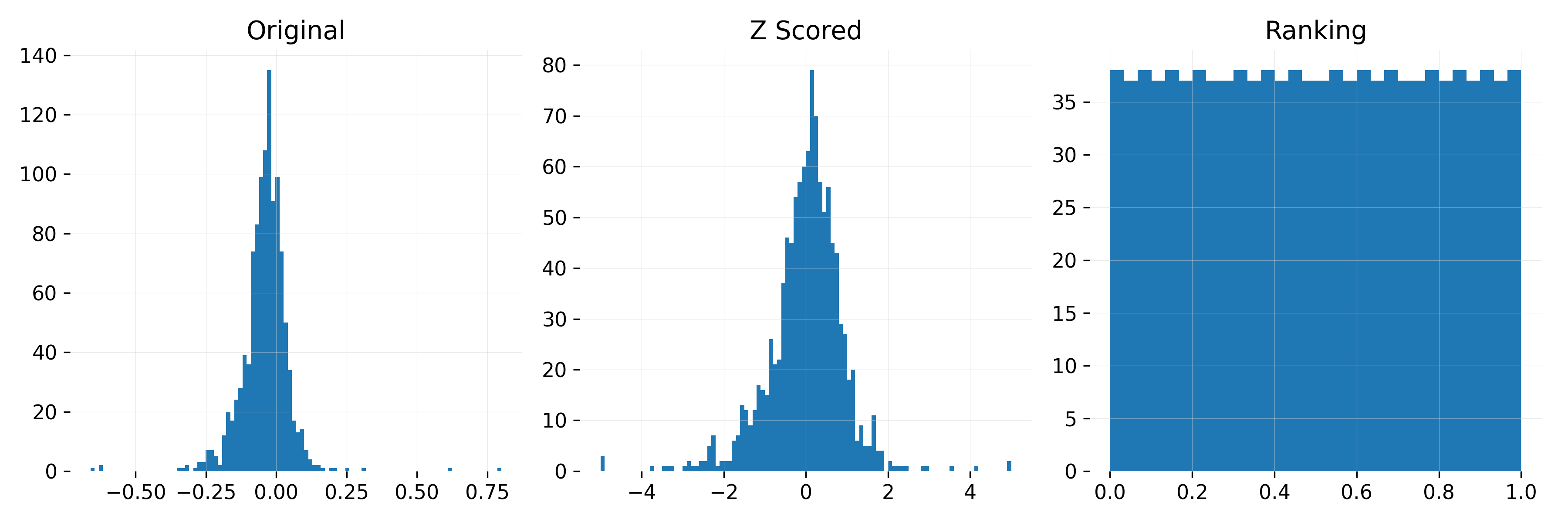
Figure 1: Effect of normalization on 20-day return distribution. Left: Original data Middle: Z-scored Right: Ranked between 0 and 1.
Choosing the Right Normalization Method
How I normalize features has a big impact on how the model interprets stock differences. The choice between z-scoring and ranking depends on what I want the model to focus on.
- Z-scoring keeps magnitude differences intact, which helps when the strength of a signal matters. But it’s more sensitive to distribution shifts over time.
- Ranking is more stable and removes extreme outliers since values are always mapped to a uniform distribution. But it also discards information about the magnitude of differences between stocks.
Both methods make sure stocks are processed in a comparable way on any given day, but they emphasize different aspects of the data.
Evaluating the Impact of Normalization
To see if normalization improves results I compare three approaches:
- Using raw unnormalized features
- Applying z-scoring across all stocks
- Using ranking across all stocks
If normalization improves performance the next step is to refine how I apply it,especially to the target label.
Should the Target Label Be Normalized by Sector?
Normalizing features ensures consistency over time, but what about the target label? Instead of normalizing returns across all stocks, I test whether normalizing them within each sector improves results while keeping all other features globally normalized.
- Global normalization applies the same normalization across the full stock universe
- Sector-specific normalization adjusts returns within each sector while keeping all other features globally normalized
My hypothesis is that sector-normalizing the target label might help by preventing cross-sector differences from distorting the model’s learning. Stocks in different industries often have structurally different return profiles, so this adjustment could make return comparisons more meaningful. Whether this actually improves performance is something I want to find out.
Handling Missing Data
Some models (like decision trees) handle missing data automatically, but others don’t. To keep things simple, I use:
- Forward fill: Use the last known value if past data exists
- Cross-sectional mean imputation: If no past data is available, replace the missing value with the sector average for that day
- Default values: For z-scoring, set missing values to 0. For ranking, set missing values to 0.5 (midpoint of the ranking scale)
This approach is simple and works well for now.
Modeling the Cross-Sectional Normalized Score
At the core of this strategy, I’m building a model to predict a stock’s cross-sectional normalized score—could be its Sharpe ratio, return, or another performance measure. I think of this as a function mapping available information at time $t$ to an expected score at $t+1$. To make stocks comparable, the score is normalized in the cross-section before modeling.
Mathematically, I assume there exists a function $g(\cdot)$ such that:
\[s_{i,t+1} = g(\mathbf{z}_{i,t}) + \epsilon_{i,t+1}\]where $s_{i,t+1}$ is the true cross-sectional normalized score for stock $i$ at time $t+1$, $z_{i,t}$ is a vector of predictor variables for stock $i$ at time $t$, and $\epsilon_{i,t+1}$ is the error term.
The goal is to approximate $g(\cdot)$ using historical data. This function follows two key principles:
- It leverages the entire panel of stocks—the same functional form applies universally
- It depends only on stock-specific features at time $t$. While some features contain past information (like return over the past 20 days), these are explicitly engineered rather than dynamically learned. The model doesn’t learn interactions between different stocks.
Ridge Regression as a Baseline
To estimate $g(\cdot)$, I use Ridge Regression—a simple but effective baseline, especially when predictors are highly correlated. It solves:
\[\underset{\boldsymbol{\beta}}{\min} \frac{1}{n} \sum_{i=1}^n (s_{i,t+1} \mathbf{x}_i^\top \boldsymbol{\beta})^2 + \lambda \sum_{j=1}^p \beta_j^2\]where the second term $\lambda \sum_{j=1}^p \beta_j^2$ regularizes the coefficients to prevent instability.
Ridge is a good choice here because:
- Stocks with similar characteristics often exhibit collinearity, and Ridge helps stabilize coefficient estimates
- The regularization term shrinks extreme values, reducing sensitivity to noise
- It provides a simple reference point before exploring more complex models
The model is estimated using historical data, and to assess its effectiveness, I apply an expanding walk-forward validation, which I explain below.
Expanding Walk-Forward Validation
To see how well the model holds up over time, I use an expanding walk-forward validation. The idea is simple:
- Start with a 3-year burn-in period—the model isn’t tested yet; it just learns from the data
- Update the model every 2 years—each time, I add the latest data and refit the model
- Keep expanding the dataset—older data stays in, and new data gets added
With stock data, I’ve always found that more historical data is better. The signal-to-noise ratio is low, so keeping as much information as possible helps the model find the signal in all the noise.
A rolling validation window could work, but it discards older data that might still be valuable. In my experience, an expanding window works better because it lets the model pick up long-term relationships, leading to more stable predictions.
For hyperparameter tuning, I could split the training set into separate train and validation sets. But honestly, I’ve never found this to be worth the extra time. Optimizing hyperparameters can take a while, and in most cases, default values that make sense are already a good starting point.
Below is a schematic of the expanding walkforward approach:
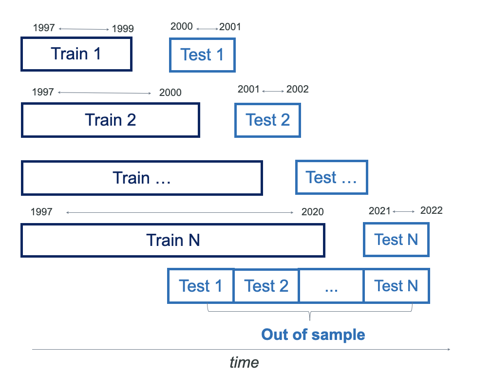
Figure 2: Expanding walkforward validation process.
Portfolio Construction
Once I have stock rankings, I build a long-short portfolio:
- I go long on the 75 stocks with the highest scores
- I short the 75 stocks with the lowest scores
This approach is robust across different portfolio sizes—whether using 50, 100, or 150 stocks.
To keep risk under control, I use volatility targeting:
- Higher-volatility stocks get smaller weights
- Lower-volatility stocks get larger weights
This ensures the portfolio maintains a stable risk profile instead of being dominated by a few volatile names.
For more detail on my portfolio construction process, check out my previous article.
Results
To evaluate different modeling choices I tested 10 model variations combining:
- 5 normalization methods: Raw Z-score (global & sector) Ranking (global & sector).
- 2 target labels: Sharpe Ratio (SR 20) and Return (Return 20).
- A combined strategy (“Combo”) which equally weights all strategies.
To ensure a fair comparison, all strategies are scaled to 10% volatility. The goal is to understand how normalization, sector adjustments, and target labels affect performance. Figure 3 shows cumulative returns across all strategies (without labels, to keep things interesting).
While all models deliver positive returns, there are clear differences in performance.
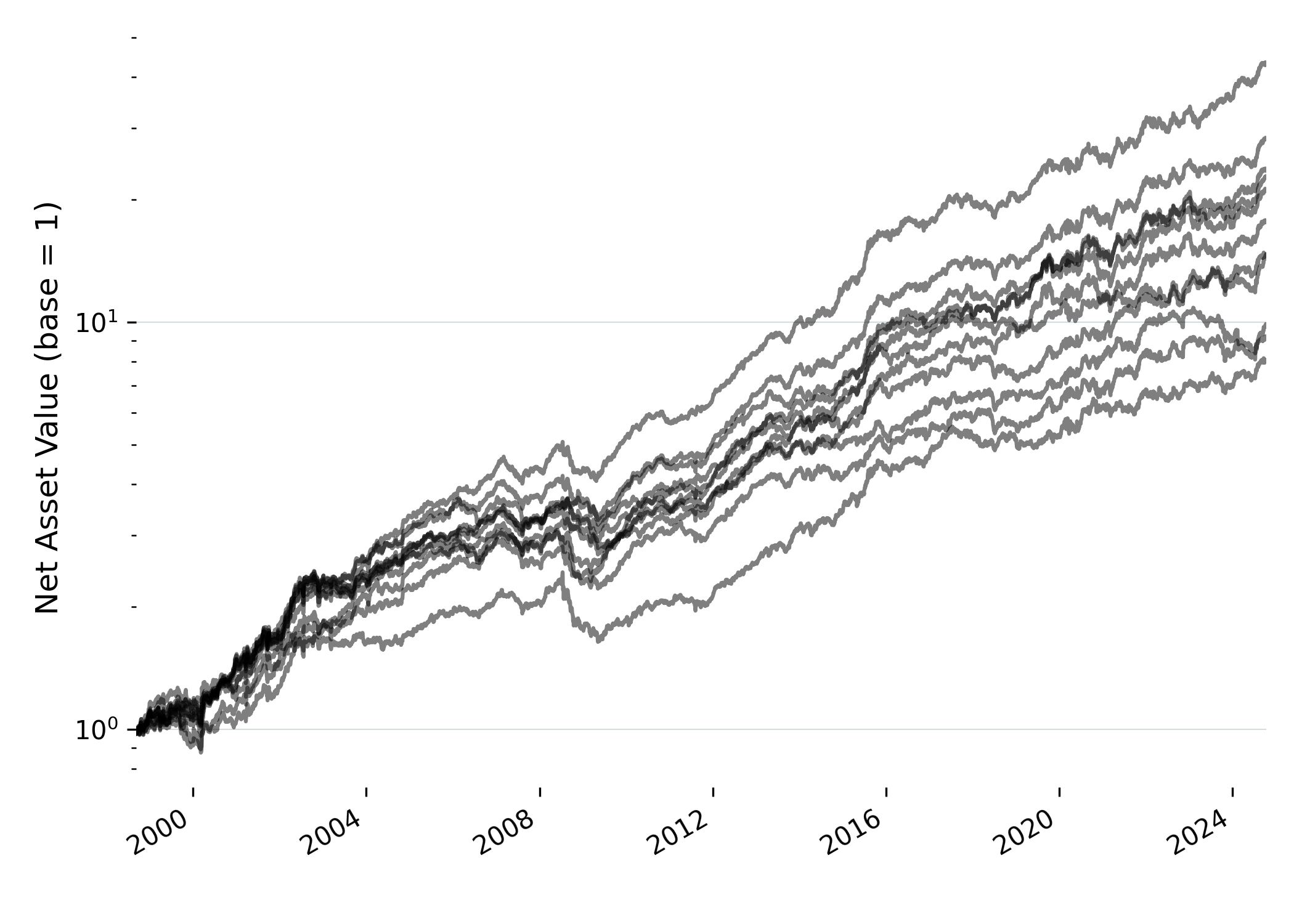
Figure 3: Cumulative returns of all strategies scaled to 10% volatility.
Figure 4 shows how different normalization methods, sector adjustments, and target label choices affect Sharpe ratios across the models. It compares z-scoring, raw features, and ranking, and also looks at the effect of normalizing within sectors versus globally. Plus it shows how using Sharpe ratios or raw returns as the target label changes things.
First off, normalization is pretty clear: z-scoring works best, then ranking, and raw features consistently underperform. I was honestly expecting ranking to be the top performer because it’s supposed to stabilize things, but it seems like it might also take out some useful signals. Z-scoring holds onto more of that valuable information, which is why it does so well. Raw features just add noise, so they end up being the weakest choice.
Then sector adjustment comes in and has an even bigger impact. Normalizing within sectors really improves Sharpe ratios compared to global normalization. It makes sense because comparing stocks within the same sector gives us more relevant context. By normalizing within sectors, I’m making sure that sector-wide noise doesn’t interfere with the real signals, so the rankings are more stable.
Lastly, the target label is by far the most important factor. When I use Sharpe ratios as the target, the models consistently perform better than when I use raw returns. This is no surprise—it’s easier to predict volatility than raw returns, so Sharpe ratios give more reliable risk-adjusted performance.
To sum it up: while normalization and sector adjustments matter, the key takeaway is the target label. Sharpe ratios beat raw returns every time, and sector normalization makes the rankings a lot stronger.
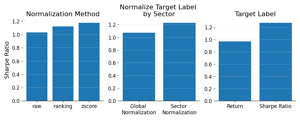
Figure 4: Sharpe Ratio performance across key modeling choices.
Normalization Effects Depend on the Target Label
Digging a bit deeper, Figure 5 shows the effect of normalization conditioned on the target label.
For Return 20 models, normalization had a smaller effect, but ranking and z-scoring still outperformed raw features. Interestingly, z-scoring has regained popularity in recent years.
For Sharpe Ratio models, the impact of normalization was stronger. Z-scoring was clearly the best performer, followed by ranking, then raw features.
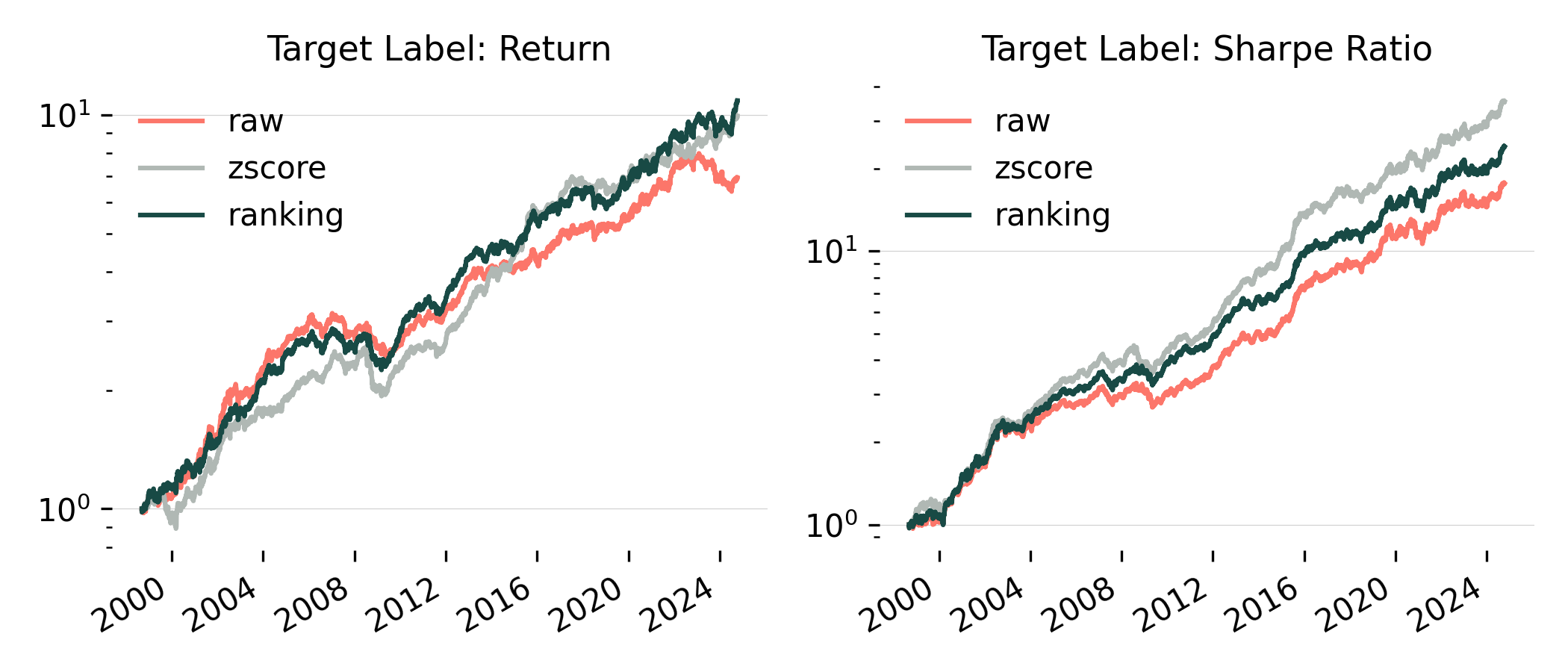
Figure 5: Cumulative return of different normalization methods conditioned on the target label. Volatility is set at 10% for all strategies.
Key Takeaways
- Normalization improves signal stability, helping models generalize better
- Sector-based adjustments on the target label refine comparisons, preventing large sector-specific biases
- Target label choice affects robustness—Sharpe ratio-based models perform better
The “Combo” Strategy Holds Up Well
I was surprised to see that the “Combo” strategy performed really well, coming in second for Sharpe ratio (you can see it in Table 1). Instead of picking just one top model, it weights all strategies equally, and still ended up second overall.
Even without fine-tuning, blending multiple models helped smooth the performance and made it more stable. It’s pretty clear to me that diversifying across models can outperform just sticking with a single “best” model.
Full Performance Breakdown
To quantify these findings here’s the performance breakdown across models:
| Model | Return (ann.) | Volatility (ann.) | Sharpe Ratio | Max Drawdown |
|---|---|---|---|---|
| SR Z-Score By Sector | 12.24% | 7.94% | 1.54 | 16.09% |
| Combo | 8.99% | 6.62% | 1.36 | 15.19% |
| SR Z-Score Global | 10.68% | 8.30% | 1.29 | 18.39% |
| SR Ranking By Sector | 9.95% | 7.83% | 1.27 | 13.94% |
| SR Ranking Global | 10.40% | 8.41% | 1.24 | 15.93% |
| SR Raw Global | 9.76% | 8.39% | 1.16 | 15.89% |
| Return Ranking By Sector | 8.14% | 7.50% | 1.09 | 15.96% |
| Return Z-Score By Sector | 8.07% | 7.43% | 1.09 | 19.37% |
| Return Raw Global | 6.95% | 7.54% | 0.92 | 18.99% |
| Return Ranking Global | 6.48% | 7.26% | 0.89 | 18.86% |
| Return Z-Score Global | 6.44% | 7.67% | 0.84 | 25.95% |
Table 1: Performance metrics across different modeling choices ranked by Sharpe Ratio in descending order. Results exclude transaction costs and slippage.
Conclusion
Sector normalization (target label), normalization method, and target label choice all had a meaningful impact on performance:
- Sector normalization was a game-changer—comparing stocks within their sector led to major improvements
- Normalization method mattered more than expected—z-scoring outperformed ranking, contradicting my initial intuition
- Sharpe ratio models consistently outperformed return-based models, reinforcing the importance of risk-adjusted metrics
Instead of searching for a single best model, it may be smarter to combine perspectives. The “Combo” strategy showed that diversifying across models stabilizes results, even without fine-tuning.