Stock Ranking with Boosting
Introduction
This is the third post in a series on stock ranking. The first used a simple low-volatility factor. The second combined multiple features with Ridge regression. Now I want to see if a non-linear model can do better.
The setup stays the same: Russell 1000 stocks, ranked daily, long the top 75, short the bottom 75, with volatility-targeted sizing and tranched rebalancing. Only the model changes.
Why LightGBM
Ridge learns fixed weights for each feature. That’s limiting. Markets aren’t linear, and there are patterns Ridge can’t capture: a feature like volatility might only matter when combined with momentum, or extreme values might behave differently than moderate ones.
Gradient boosting handles this naturally. It builds predictions by stacking small decision trees, each one correcting the mistakes of the previous. The result is a model that can learn interactions and non-linearities without me having to specify them.
I’m using LightGBM specifically because it’s fast. XGBoost and CatBoost would probably give similar results, but LightGBM trains quicker on large datasets. For rolling estimation, speed matters.
Performance
The results are strong.
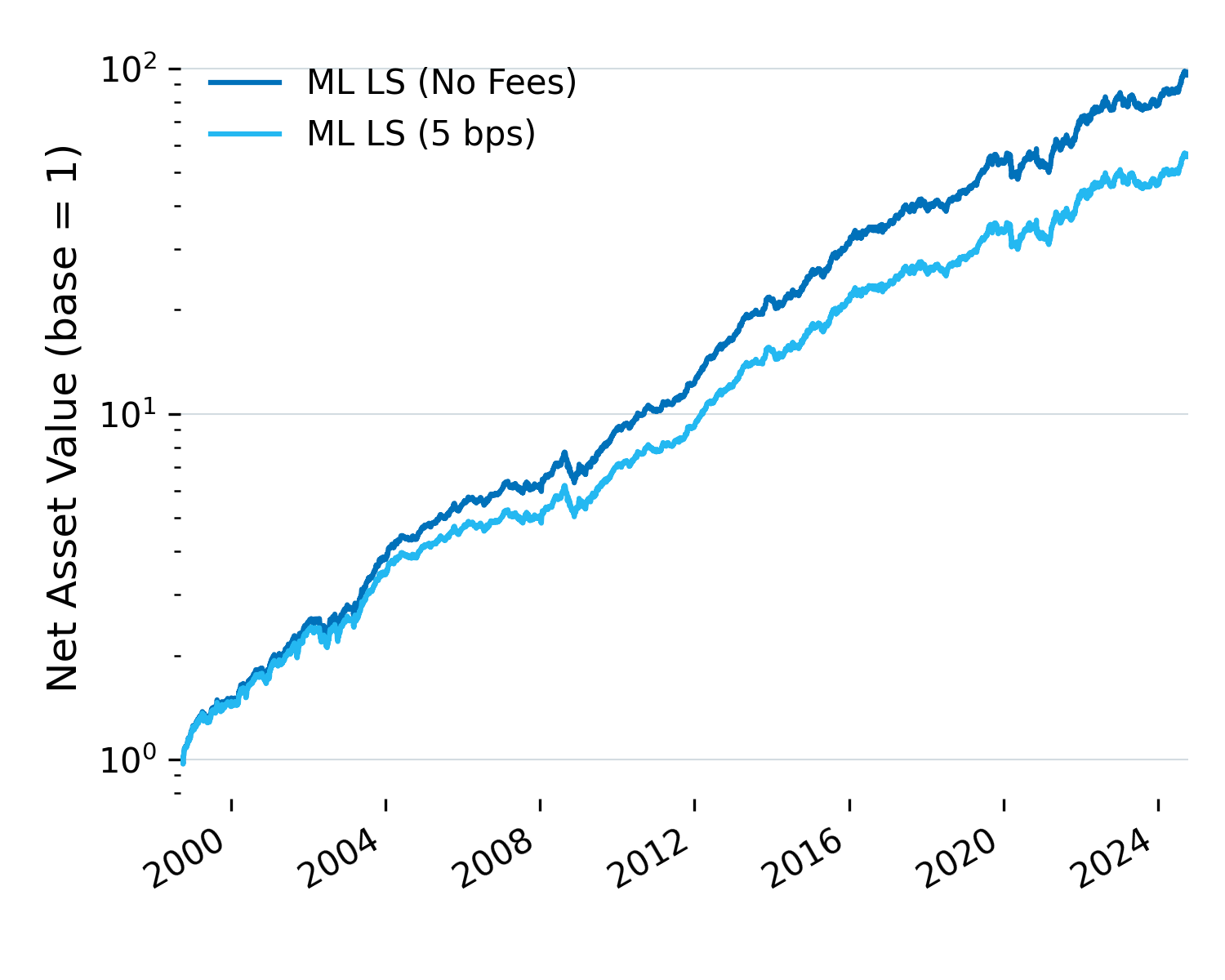
Figure 1: LightGBM strategy performance, before and after transaction costs.
| Metric | Short Leg | Long Leg | L/S (No Fees) | L/S (Fees) | Russell 1000 |
|---|---|---|---|---|---|
| Return (Annualized) | 1.46% | 12.48% | 12.33% | 10.69% | 7.29% |
| Volatility (Annualized) | 9.95% | 10.54% | 6.67% | 6.69% | 19.58% |
| Sharpe Ratio | 0.15 | 1.18 | 1.85 | 1.60 | 0.37 |
| Max Drawdown | 30.78% | 31.10% | 13.79% | 13.97% | 56.88% |
| Max Time Underwater | 1,619 days | 599 days | 234 days | 265 days | 1,666 days |
Table 1: Performance with and without transaction costs (5 bps per trade).
After fees, the strategy returns 10.7% annually with ~7% volatility, giving a Sharpe of 1.60. Drawdowns stay around 14%, and recovery is relatively quick.
Both legs do their job. The long leg returns 12.5%, well above the Russell 1000’s 7.3%. The short leg returns just 1.5%, meaning those bottom-ranked stocks underperform as intended. That’s the clean separation you want in a ranking strategy.
Signal Quality
Before portfolio construction, how well does each model actually rank stocks?
Each day, I compute the Spearman correlation between predicted scores and realized 20-day forward Sharpe ratios. This measures raw signal quality, independent of position sizing or rebalancing.
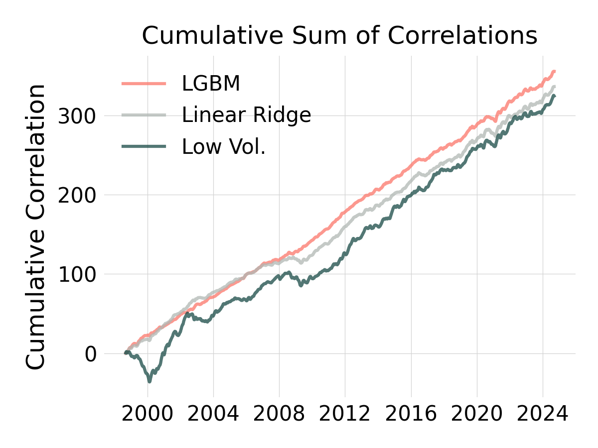
Figure 2: Cumulative Spearman correlation between model signals and realized rankings.
| Metric | Low Volatility | Ridge | LightGBM |
|---|---|---|---|
| Mean | 4.96% | 5.14% | 5.43% |
| Standard Deviation | 14.39% | 8.70% | 7.03% |
| Sharpe Ratio | 0.34 | 0.59 | 0.77 |
Table 2: Daily signal quality metrics.
Correlations around 5% might seem low, but that’s normal for financial data. The key is consistency. LightGBM delivers a more stable signal with less variance and a higher signal-level Sharpe. Even weak signals compound into meaningful performance when applied systematically.
Comparing All Three
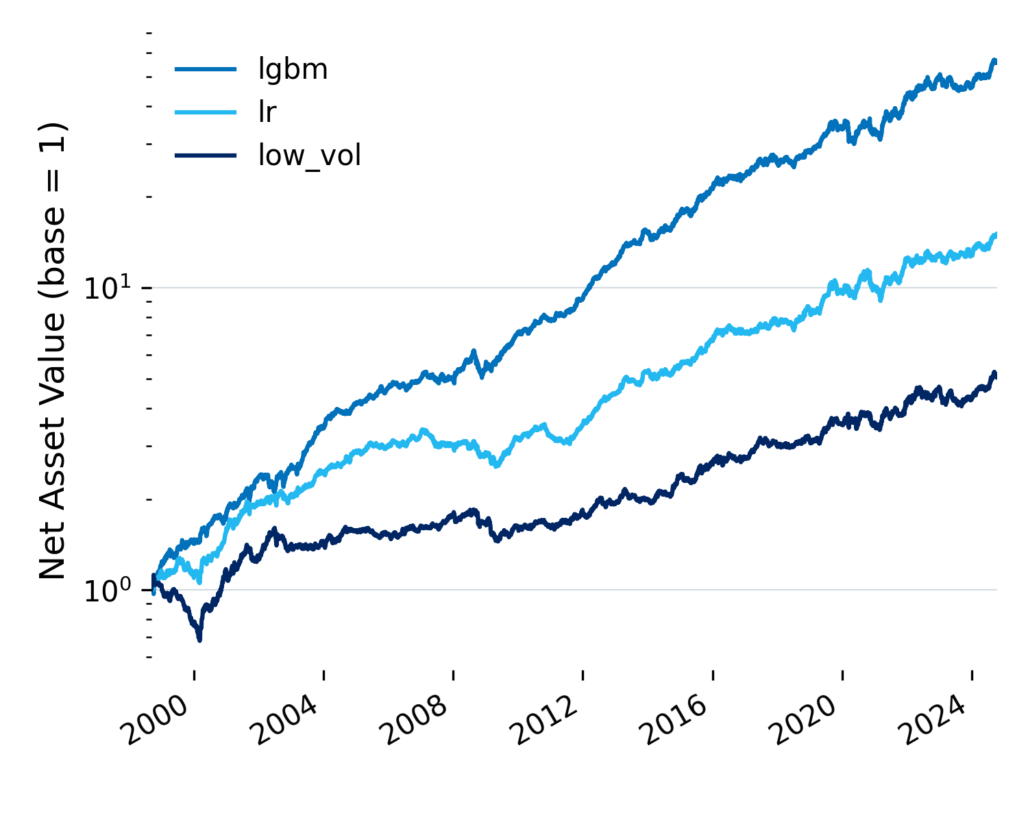
Figure 3: Full sample performance (1997-2024).
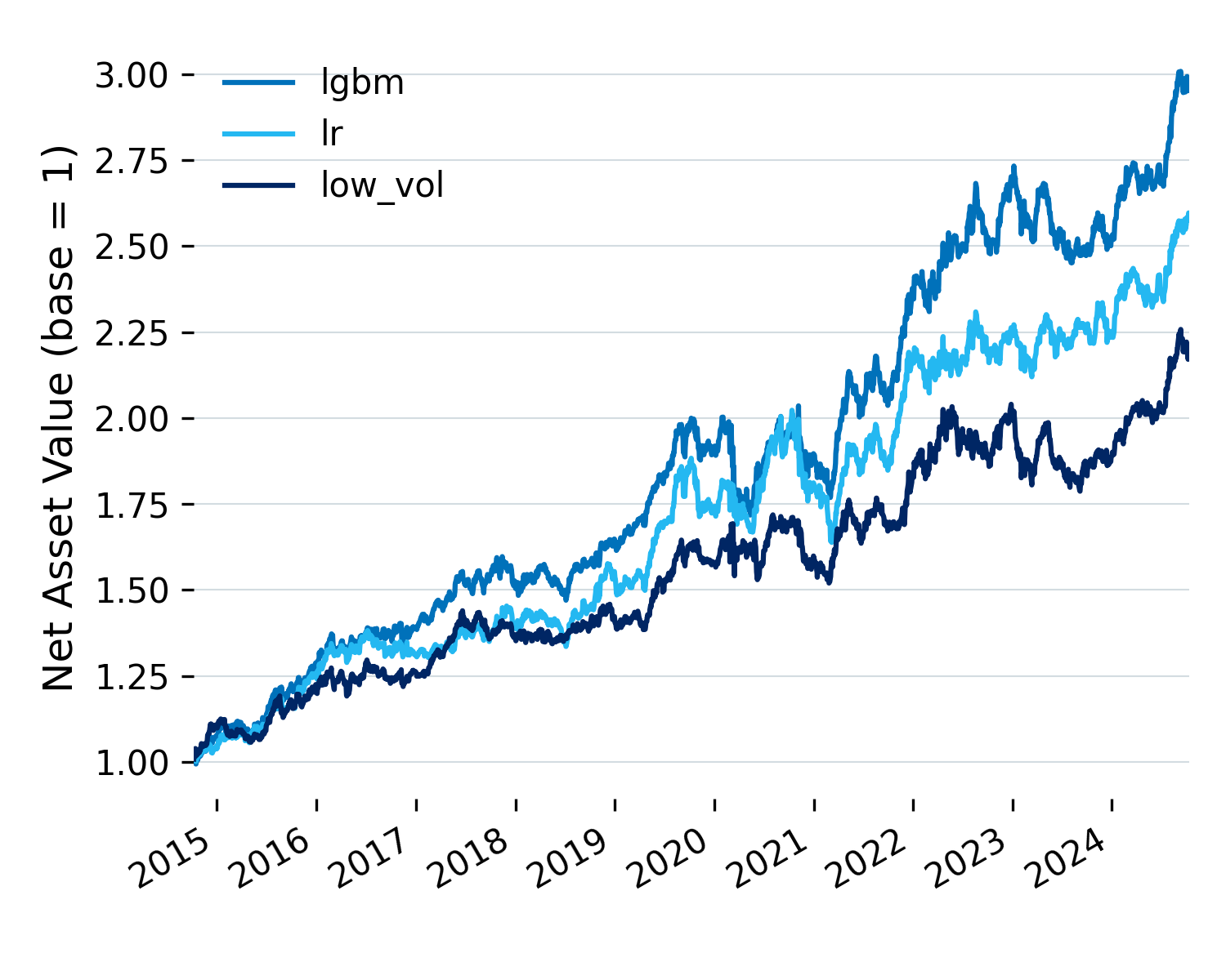
Figure 4: Last decade (2015-2024).
| Metric | Low Vol (Full) | Ridge (Full) | LGBM (Full) | Low Vol (10Y) | Ridge (10Y) | LGBM (10Y) |
|---|---|---|---|---|---|---|
| Return (Ann.) | 5.62% | 8.76% | 11.68% | 7.94% | 8.91% | 9.33% |
| Volatility (Ann.) | 8.67% | 7.98% | 7.09% | 9.76% | 8.91% | 8.17% |
| Sharpe Ratio | 0.67 | 1.09 | 1.59 | 0.83 | 1.00 | 1.13 |
| Max Drawdown | 35.27% | 20.18% | 13.71% | 12.11% | 17.07% | 11.69% |
| Max Time Underwater | 844 days | 862 days | 297 days | 350 days | 307 days | 297 days |
Table 3: Performance comparison across all three approaches.
LightGBM leads across nearly every metric. Higher returns, lower volatility, smaller drawdowns, faster recovery.
But the last decade tells a different story. Performance has softened across the board. LightGBM’s Sharpe drops from 1.59 to 1.13, and Ridge isn’t far behind at 1.00. The edge has narrowed.
What’s going on? Has the market become more efficient? Are the features decaying? Is the model overfitting to older regimes? These are open questions.
Conclusion
LightGBM works better than Ridge, which works better than raw volatility. The progression makes sense: more flexibility captures more signal.
But performance has weakened in recent years, and I don’t fully understand why. A few things I want to explore:
-
Portfolio construction: I’ve been reading Advanced Portfolio Management and The Elements of Quantitative Investing by Paleologo. Want to better understand what’s actually driving P&L and whether there’s a smarter way to size positions.
-
Features and targets: Everything here is based on price, volume, and market cap. There’s probably more signal to find, or better ways to use existing data. Also worth revisiting the prediction horizon.
-
Rethinking the objective: The current pipeline scores stocks, then allocates separately. Maybe it makes more sense to predict weights directly. The recent paper Artificial Intelligence Asset Pricing Models (Kelly et al., 2025) takes this much further, using transformers to learn the stochastic discount factor from raw panel data. Ambitious, but interesting.
More to come.